Finite-depth Lyapunov-growth estimation in GNNs

Research note · 29 September 2026

This study asks how to estimate the top finite-depth Jacobian growth rate of a trained graph neural network. It compares exact dense SVD on small cases, random full-space JVP probes, and residual-checked JVP/VJP power iteration. The experiments use tuned GCN, ChebNet, Hariri et al.'s Stable-ChebNet, and a deep feature-conditioned sheaf-diffusion baseline on homophilic, heterophilic, and barbell graph conditions.

Download the illustrated PDF report (2.7 MB) · code, configurations, and evidence

Key result

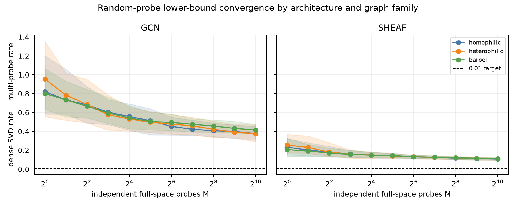
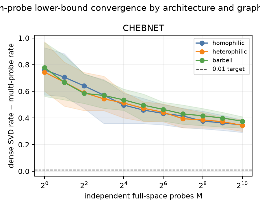
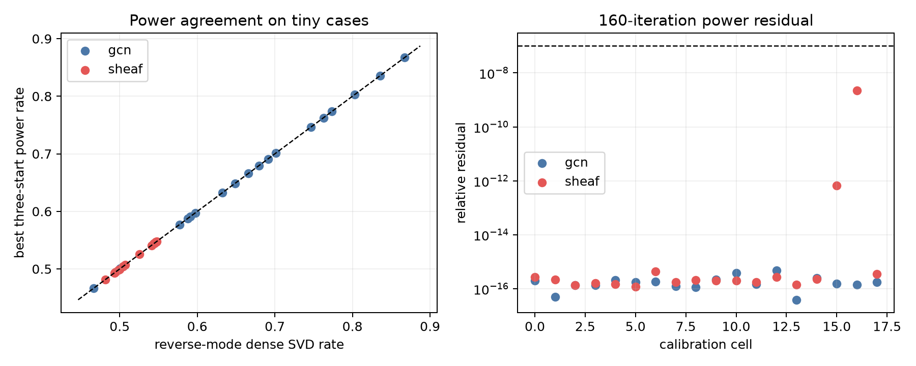
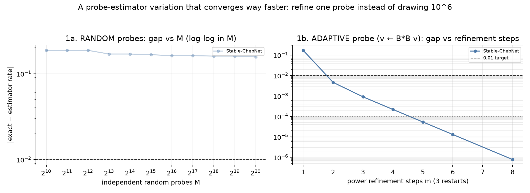
A maximum over independent random tangent probes is mathematically valid as a lower bound, but it was far too loose as a point estimator in these experiments: even 1,024 probes never reached the predeclared 0.01-per-layer accuracy target. In contrast, three-start, residual-checked power iteration on the complete Jacobian product matched exact tiny-case SVD references. The report explains why probe budgets depend on the singular spectrum and tangent dimension, rather than being a universal GNN hyperparameter.

If the estimator is restricted to forward-only JVP probes (no adjoint), the best measured estimator is the graph-aligned (smoothness-skewed) full-space multiprobe q ∝ (I + cL)^{-1}z: it beats iid probes on every cell at ~2–5× (gap@2^20 GCN 0.166 vs 0.313, ChebNet 0.154 vs 0.292, sheaf 0.045 vs 0.086 at equal wall), at microsecond marginal cost per batched probe — while forward-only refinement (v ← Bv/‖Bv‖) provably stalls at the spectral radius and never reaches the top singular rate.

The new Stable-ChebNet model-zoo entry (Hariri et al., arXiv:2506.07624v2) was evaluated with the same exact-SVD, full-spectrum, histogram, probe-convergence, timing, power-speedup, and forward-only follow-up protocols. Its exact top-rate histogram mean is 0.281, versus 0.804 (GCN), 1.024 (ChebNet), and 0.514 (sheaf), while its full products had no zero singular values in the 58 graph–signal examples. These are controlled synthetic-task results, not a full reproduction of the paper's long-range benchmark.

Random-probe gap versus number of probes for GCN and sheaf GNN — Random-probe lower-bound convergence: the gap remains substantial at 1,024 probes.

Random-probe gap versus number of probes for ChebNet — ChebNet independently reproduces the slow random-probe convergence.

Power iteration estimates versus exact dense SVD rates — On calibrated small cases, residual-checked power iteration agrees with dense SVD.

Held-out task accuracy by graph family for GCN and sheaf GNN — Task performance is reported separately: a global top rate is not a direct measure of task accuracy or oversquashing.

Datasets and input dependence

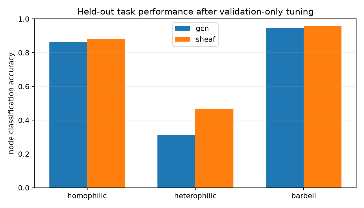
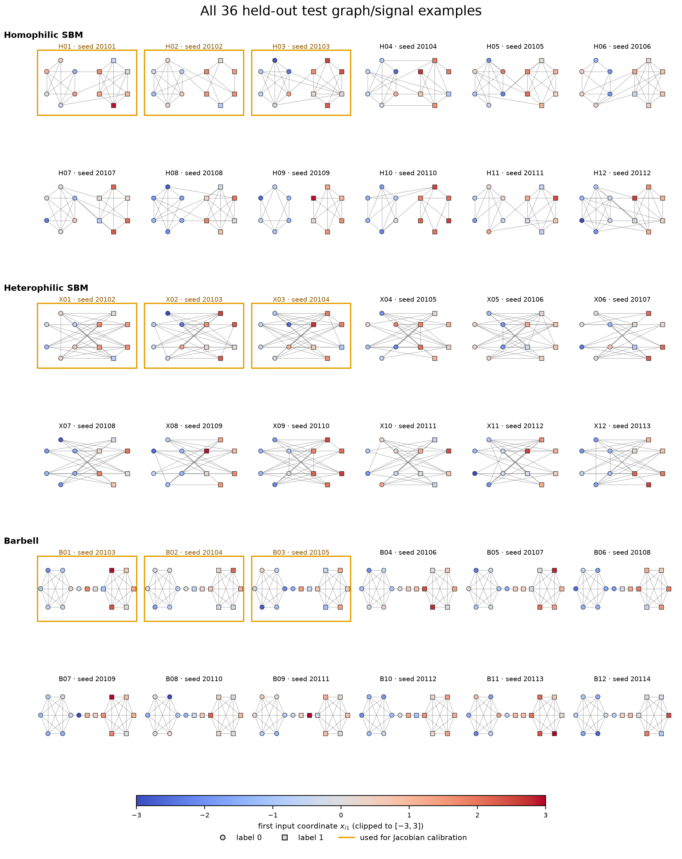
Training uses 16 balanced, 12-node homophilic contextual SBMs and validation uses six fresh graphs from the same distribution. Each node has a four-dimensional signal: a noisy class-dependent first coordinate and three noise coordinates. Hyperparameters are selected only from validation accuracy. Testing uses 12 fresh graphs from each of three conditions: matched homophilic SBMs, heterophilic SBMs with reversed edge probabilities, and 15-node barbells with a three-node bottleneck. Jacobian calibration uses the first three examples per condition for each of two model seeds. The complete split contains 58 unique graphs: 16 training, six validation, and 36 testing; Jacobian calibration reuses the first three test examples per condition, for nine unique graph/signal inputs.

The rate is computed pointwise: within a cell, the graph, feature signal, trained model, and forward trajectory are fixed; random probes vary tangent directions, not data inputs. Across cells, the report summarizes an empirical distribution over jointly generated graph/signal pairs. It therefore does not yet isolate variation in the input signal while holding a single graph fixed.

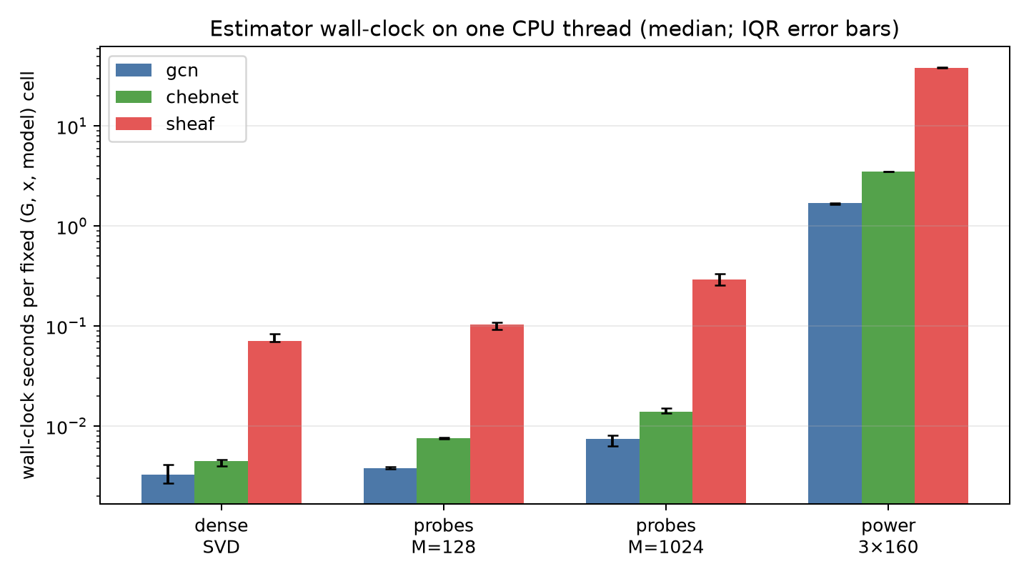
All 36 held-out test graphs with node signal values and calibration subset highlighted — All 36 test graphs. Node colour shows the first signal coordinate; gold frames mark the nine calibration inputs.

Estimator wall-clock comparison

On the tiny calibrated dimensions, dense Jacobian plus SVD was exact and fastest. Median one-thread CPU times per cell ranged from 0.003–0.071 seconds for dense SVD, 0.007–0.293 seconds for 1,024 vectorized probes, and 1.69–38.46 seconds for three-start/160-iteration power. The Stable-ChebNet timing medians were 0.0128 s dense SVD, 0.0401 s for 1,024 probes, and 9.07 s for fixed power. The fast random-probe method remained inaccurate. Dense storage scales quadratically, so the scalable recommendation remains residual-checked matrix-free power once an explicit Jacobian no longer fits.

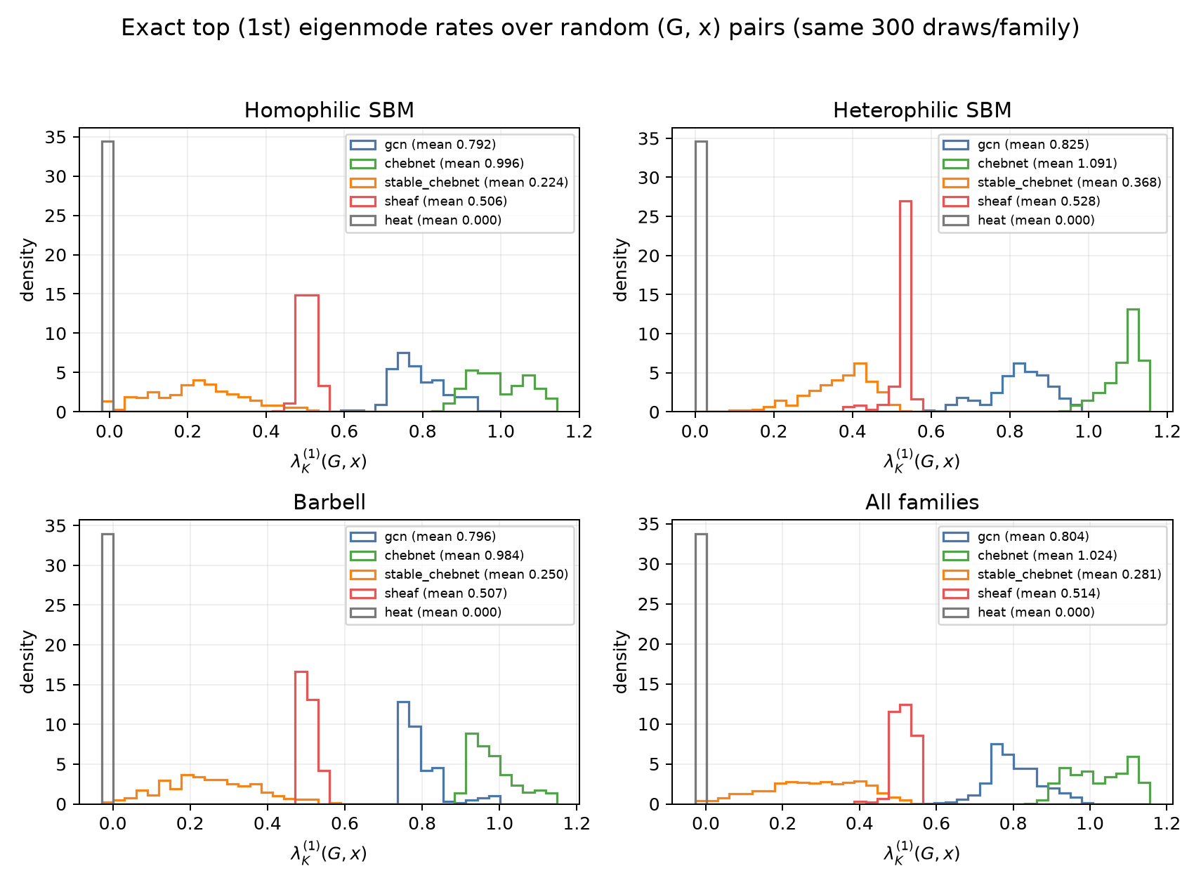
Wall-clock comparison of dense SVD, random probes, and power iteration — One-thread CPU timing on six matched cells per architecture; medians with interquartile error bars.

Lyapunov-rate histograms

Loading a trained checkpoint of each architecture and drawing the same 300 graph/signal pairs per family, the exact reverse-mode dense-SVD rate gives 900 pointwise values per model. The models are cleanly separated in this pilot: ChebNet dominates every family (mean about 0.98–1.09), GCN is intermediate (about 0.79–0.83), Stable-ChebNet is lower (about 0.22–0.37), and the deep sheaf is lowest (about 0.51–0.53). Distributions are narrow relative to their means, so the finite-depth rate meaningfully distinguishes these trained architectures, and family has a smaller effect than model choice.

The same draws are also evaluated under a non-GNN control: linear graph heat diffusion ẋ = −Lx with a stable Euler step. Its top rate is exactly 0 (mean ≈ 2.7×10⁻¹⁷): the Laplacian preserves the constant node mode and decays everything else, so heat diffusion is mass-preserving and non-expanding here. This confirms the positive GNN rates are genuine growth, not an estimator artifact.

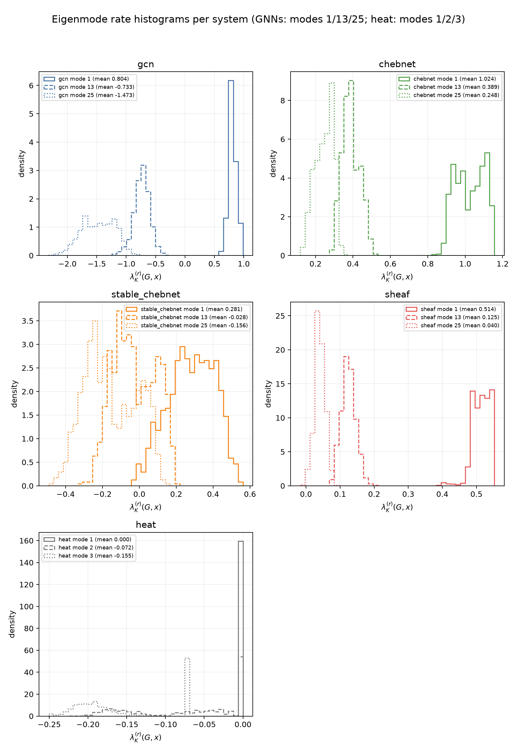
Exact Lyapunov-rate histograms for GCN, ChebNet, Stable-ChebNet, sheaf, and heat across graph families — Exact finite-depth rate distributions over random graph/signal pairs, by family and combined.

The exact estimator also returns the full singular-value spectrum, each draw giving eigenmode rates for modes 1 through 25. The GNNs are shown at widely spaced modes 1/13/25. ChebNet and the sheaf decay slowly and stay positive (ChebNet 1.024→0.389→0.248; sheaf 0.514→0.125→0.040), Stable-ChebNet decays smoothly (0.281→−0.028→−0.156), while GCN plunges negative by mode 13 (0.804→−0.73→−1.47), so growth is concentrated in just a few leading directions. Heat, evaluated on a single scalar field, keeps modes 1/2/3: mode 1 stays 0 (constant mode preserved) while modes 2/3 go negative (≈ −0.07 and −0.16), i.e. genuine contraction.

Eigenmode rate histograms per system including Stable-ChebNet at modes 1, 13, 25 — Finite-depth eigenmode rates (GNNs: modes 1/13/25 solid/dashed/dotted; heat: modes 1/2/3).

Expected empirical singular-value measures

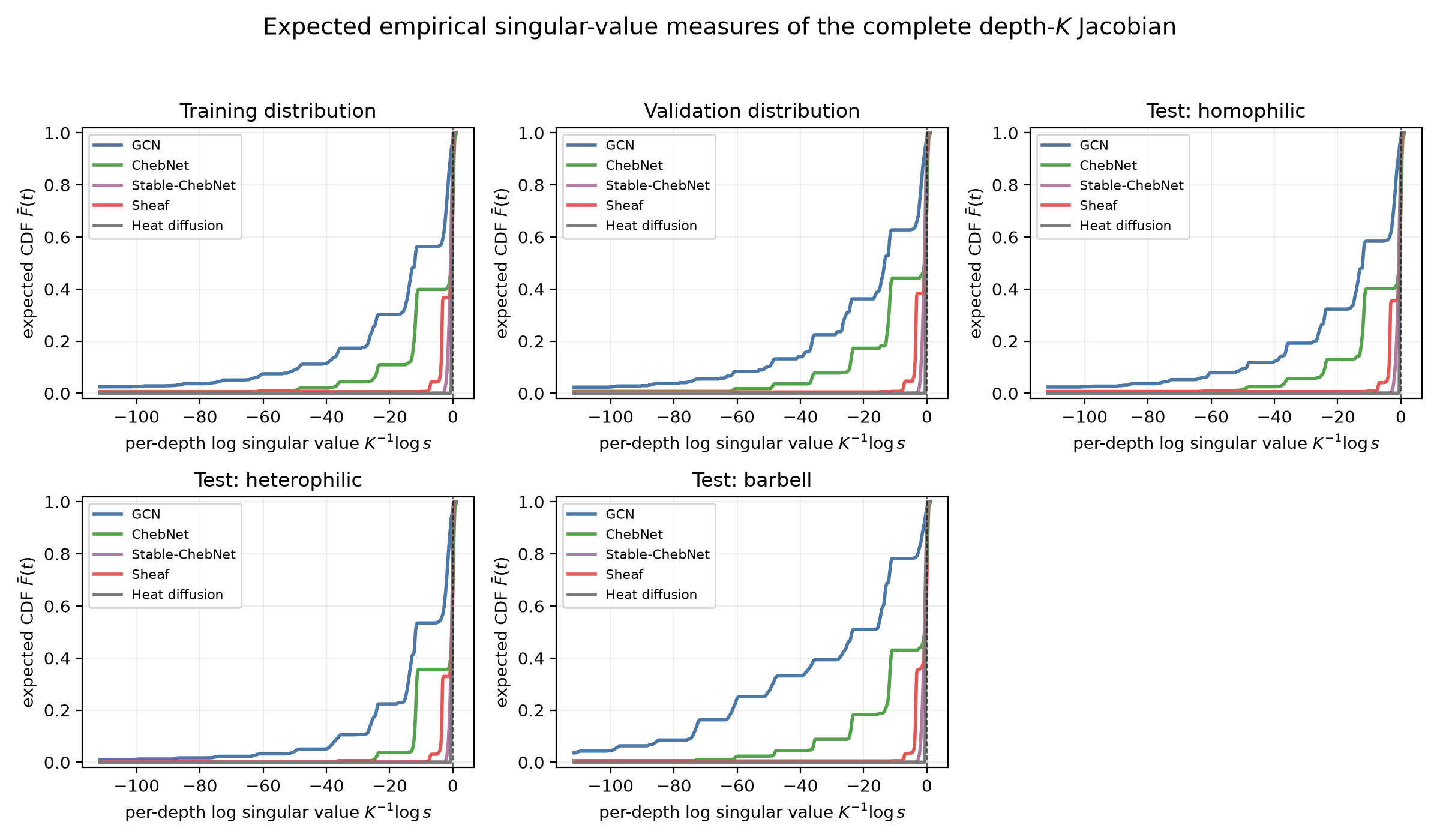
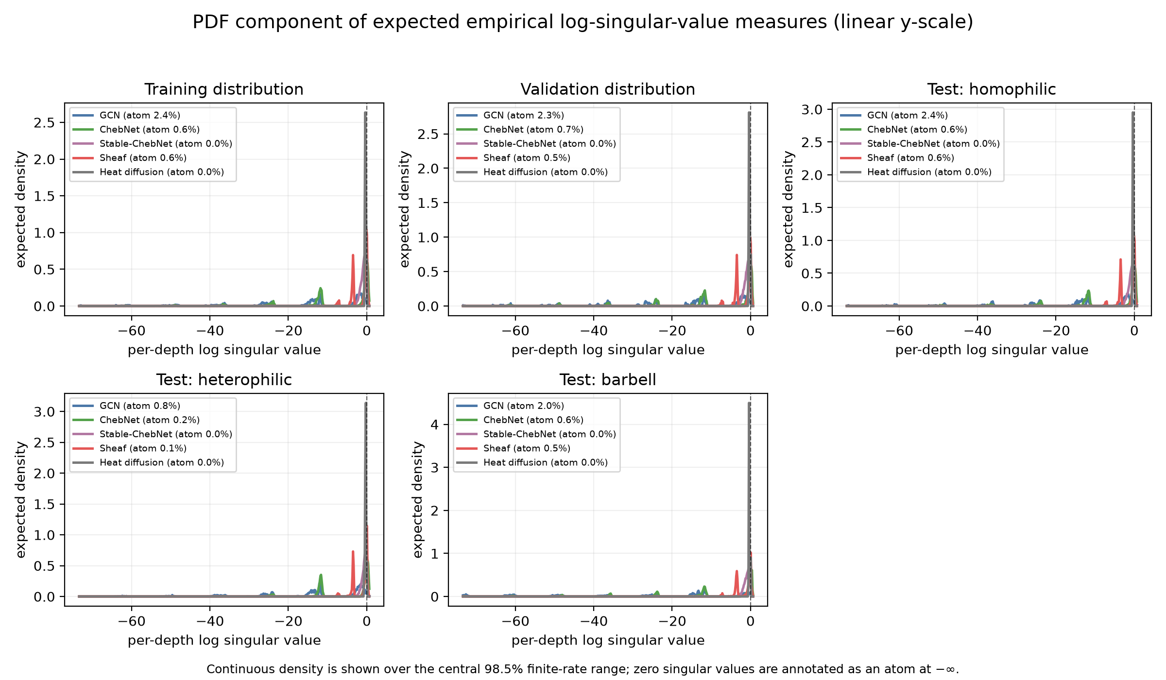
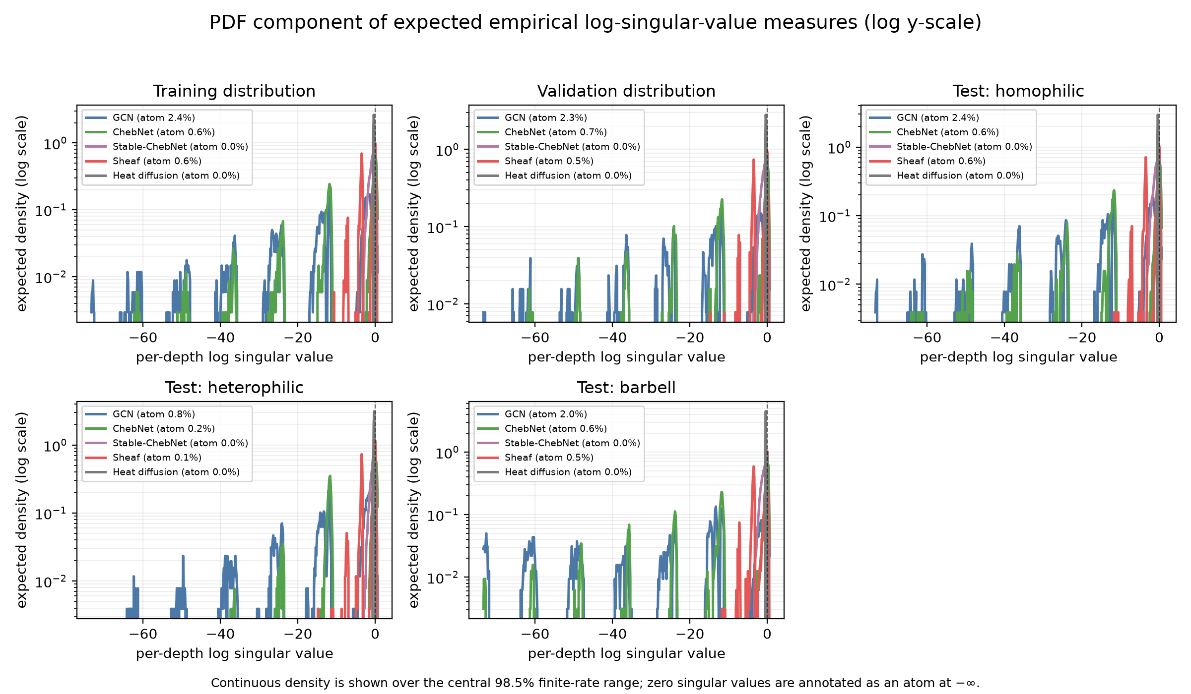
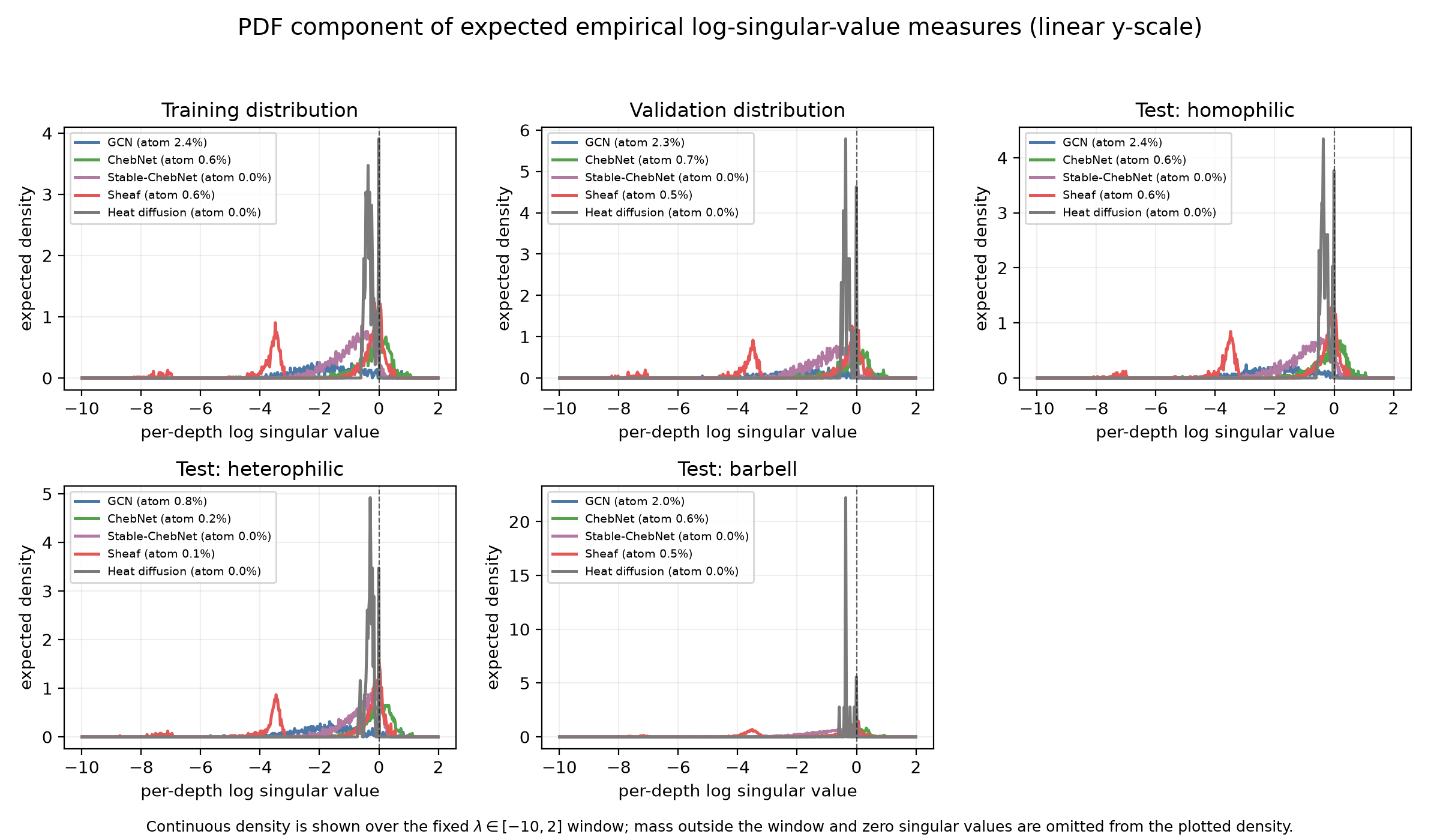
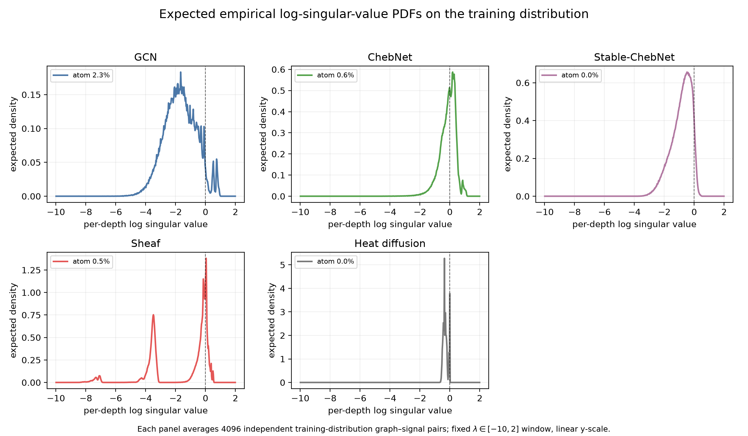
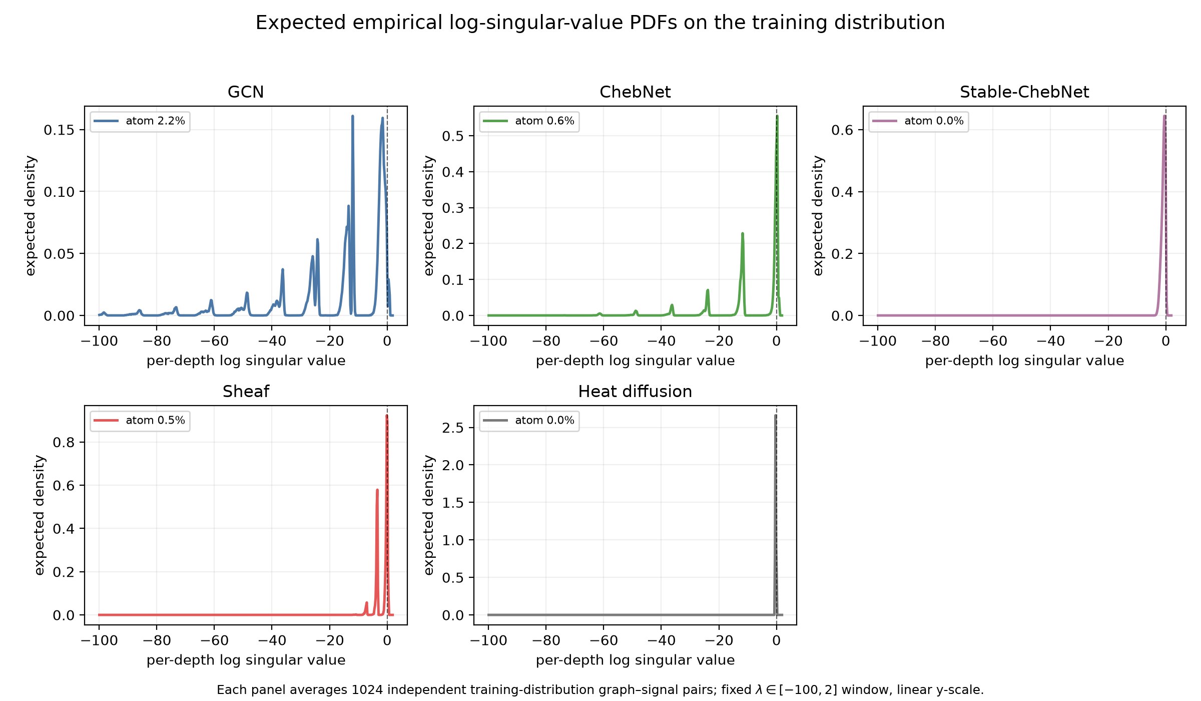
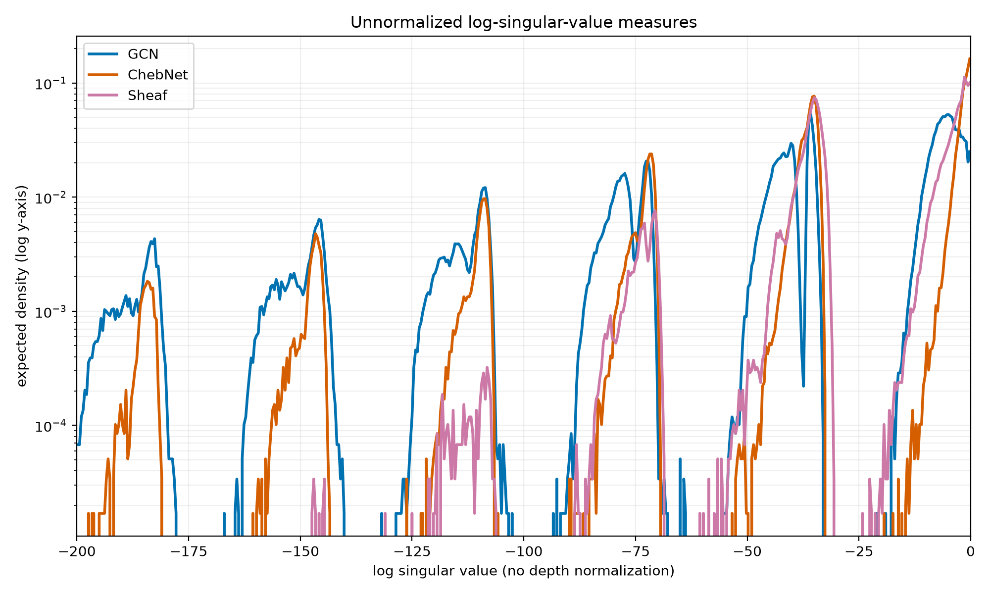
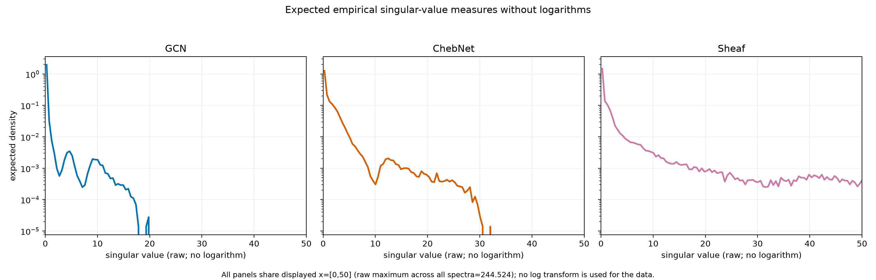
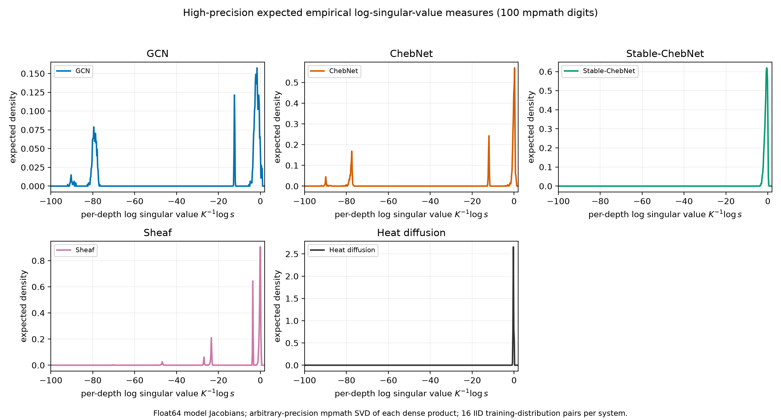
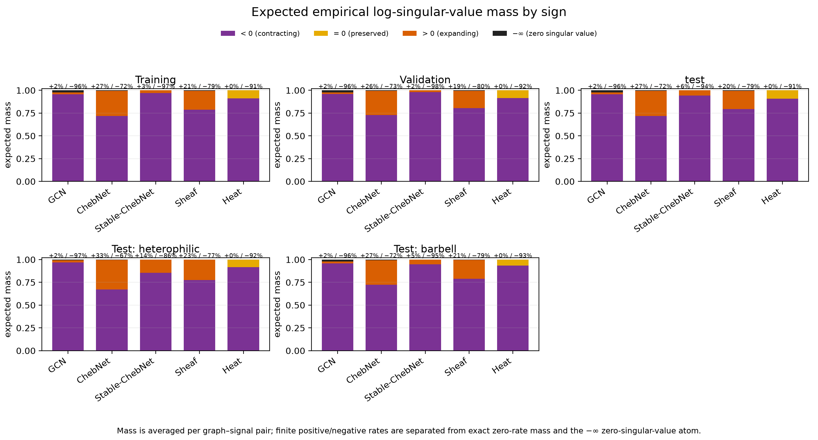
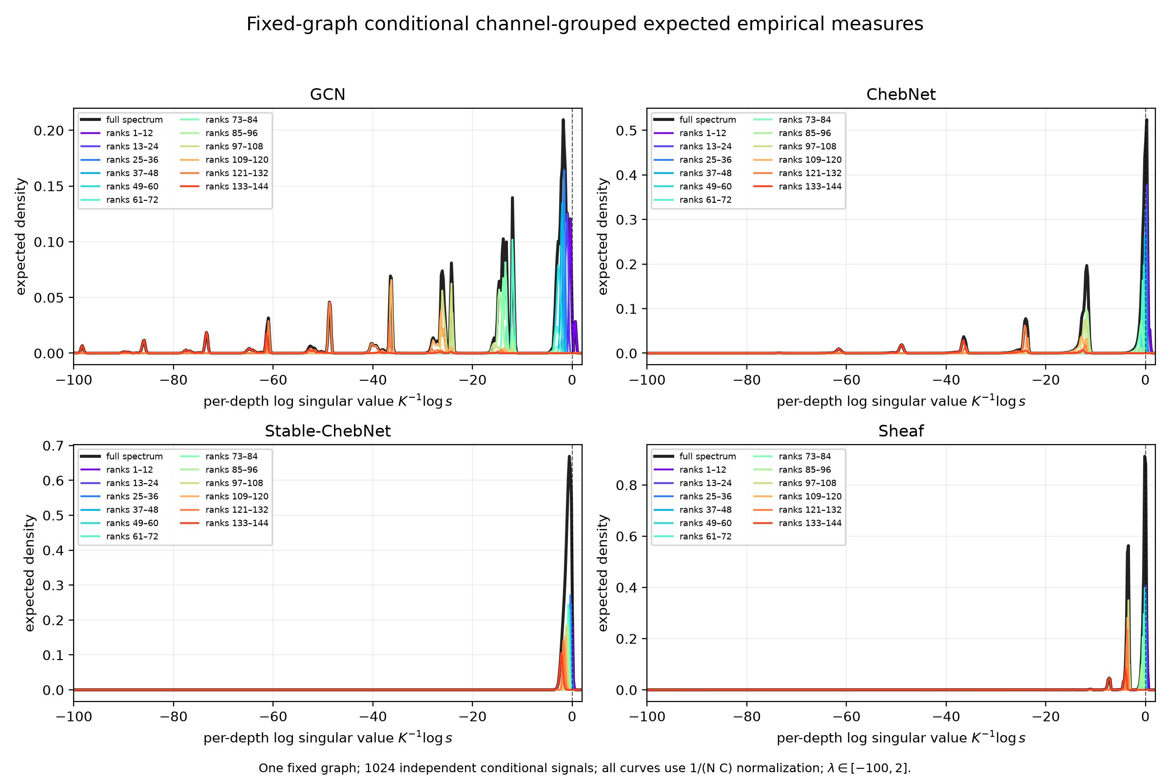
A new full-spectrum experiment forms the complete depth-K hidden-state Jacobian by explicit reverse-mode autodiff and averages each normalized empirical singular-value measure over graph–signal pairs. It covers all 16 training graphs, six validation graphs, and 36 held-out test graphs for each GNN checkpoint, plus single-channel heat diffusion on the same graph distributions. Training top-rate means are 0.777 (GCN), 0.987 (ChebNet), 0.136 (Stable-ChebNet), 0.505 (sheaf), and approximately 0 (heat), while the bulk is strongly contracting; this is a fixed-depth spectral observable, not the spectrum of an expected Jacobian or an asymptotic Lyapunov distribution.

Expected CDFs of per-depth log singular values for GCN, ChebNet, Stable-ChebNet, sheaf, and heat diffusion — Expected CDFs of the complete depth-K Jacobian spectrum across training, validation, and test distributions.

Expected probability density components of per-depth log singular values — Continuous PDF components on a linear density axis; zero singular-value atoms are annotated.

Expected probability density components on a logarithmic density axis — The same expected PDF components on a logarithmic density axis, revealing low-density tails.

Expected linear-scale spectral density restricted to Lyapunov rates from minus ten to two — Expected linear-scale density in the fixed Lyapunov-rate window −10 to 2.

Expected training-distribution spectral PDFs for all five systems using 4096 independent graph-signal pairs per system — Training-distribution spectral PDFs using 4096 independent graph–signal pairs per system.

Expected training-distribution spectral PDFs for all five systems using 1024 independent graph-signal pairs per system over rates from minus one hundred to two — Training-distribution spectral PDFs using 1024 graph–signal pairs per system in the rate window −100 to 2.

Unnormalized log singular-value densities on a logarithmic y-axis — Unnormalized log-singular-value densities for GCN, ChebNet and sheaf on [−200,0].

Raw singular-value densities without logarithms — Raw singular-value densities, computed without taking logarithms; displayed on x=[0,50] with logarithmic y-axis.

100-digit mpmath SVD precision-control expected spectra — Figure-17-style spectra from 16 samples using 100-digit mpmath SVDs of float64 Jacobians.

Synthetic GNN training loss replay — Training-loss replay for the four synthetic GNN checkpoints.

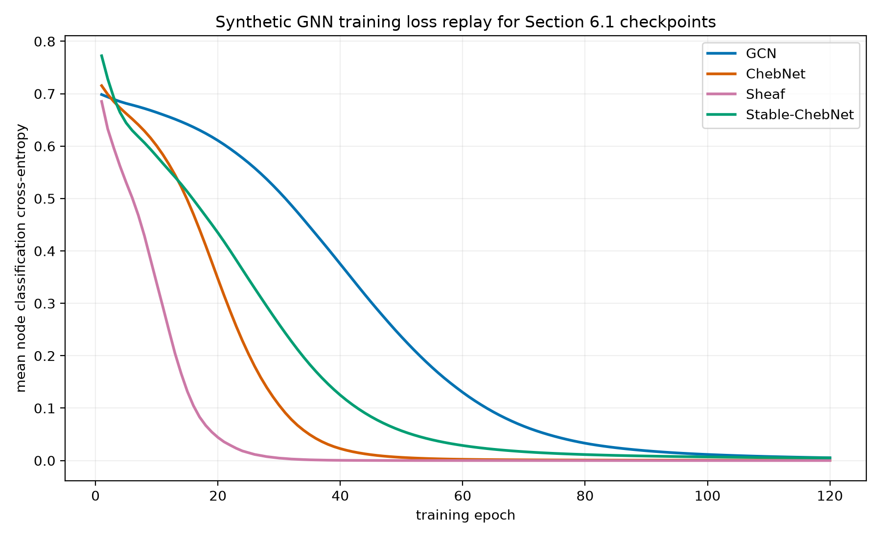
Direct checkpoint comparison confirms the replay: final training losses agree to approximately 10⁻¹⁸, and validation accuracies match exactly.

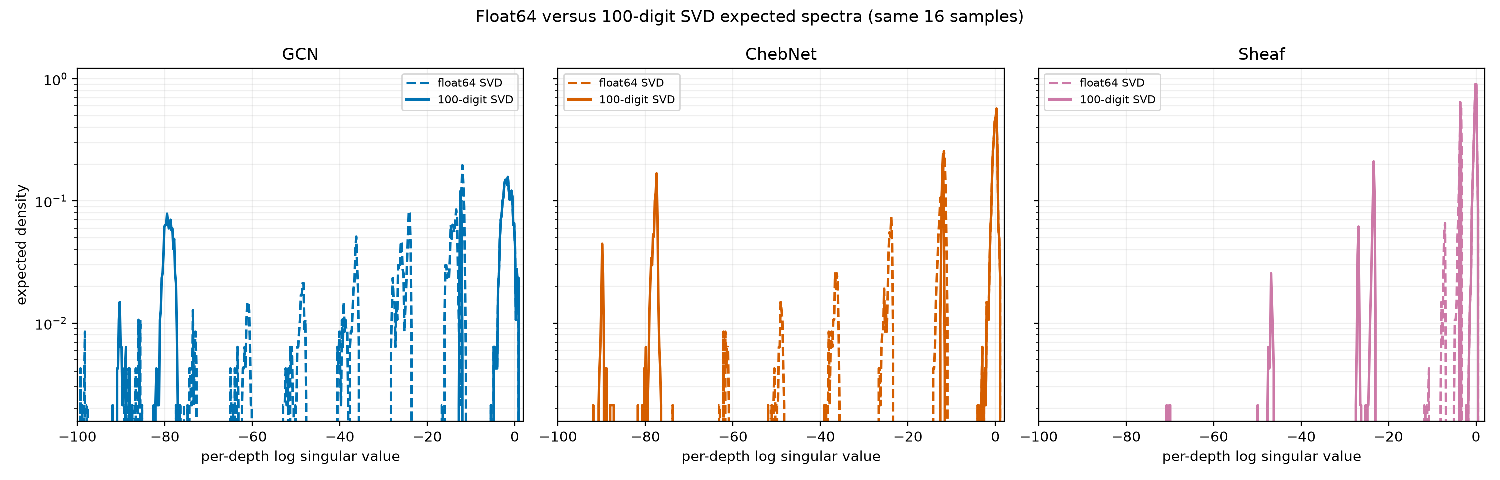
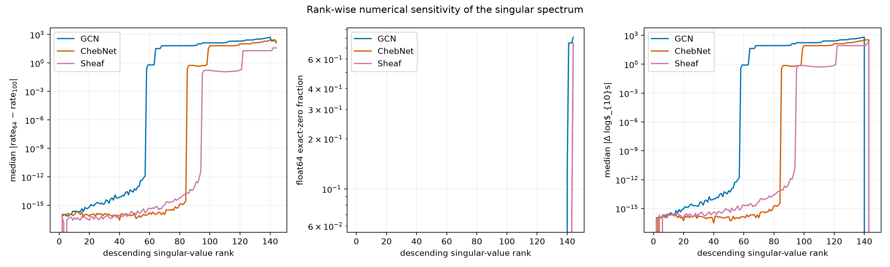
A numerical stability audit compares the float64 SVD spectra against a 100-digit mpmath recomputation: rank ordering is stable, but the deep contracting tail and near-zero classifications are precision-dependent, especially for GCN.

Float64 versus 100-digit SVD expected spectra — Float64 and 100-digit SVD expected log-rate densities on the same 16 samples.

Rank-wise numerical sensitivity — Rank-wise rate, zero-frequency and log singular-value discrepancies from the numerical audit.

Full and channel-grouped expected spectral densities for GCN, ChebNet, Stable-ChebNet, and sheaf — Full and channel-grouped expected densities with 1/(N C) normalization.

Expected spectral PDFs for four separate random initializations of each untrained GCN, ChebNet, Stable-ChebNet, and sheaf model — Expected spectra for four separate untrained random initializations per architecture over −100 to 100; legends report covered mass.

Heat diffusion expected spectral density zoomed to Lyapunov rates from minus one to zero — Heat diffusion density zoomed to the Lyapunov-rate window −1 to 0.

Mean spectral quantile profiles for the five systems including Stable-ChebNet — Mean within-example spectral quantile profiles: the bulk spectrum, not only the top mode.

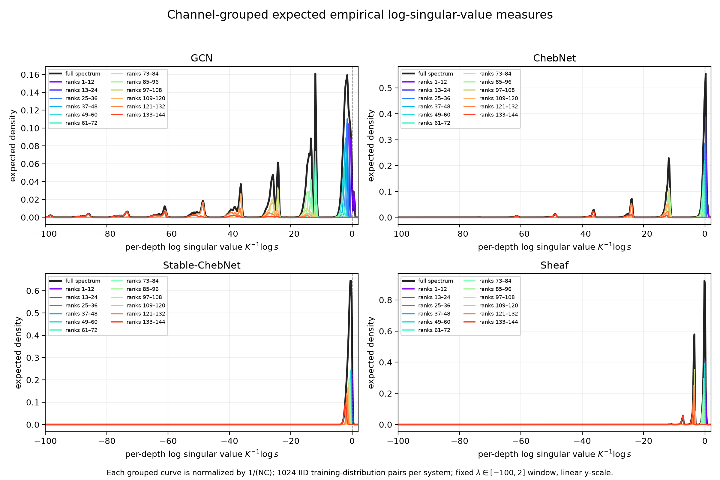
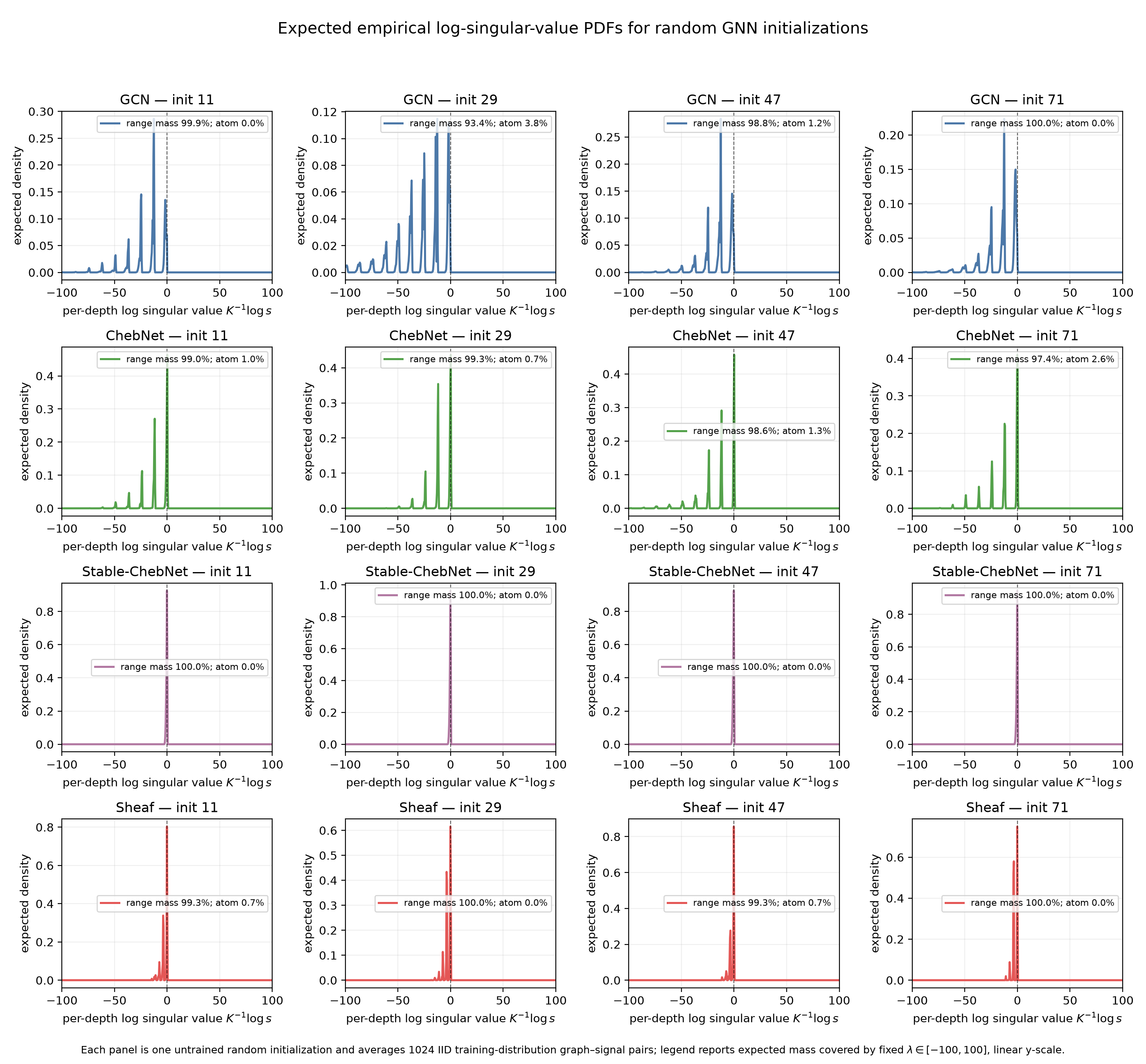
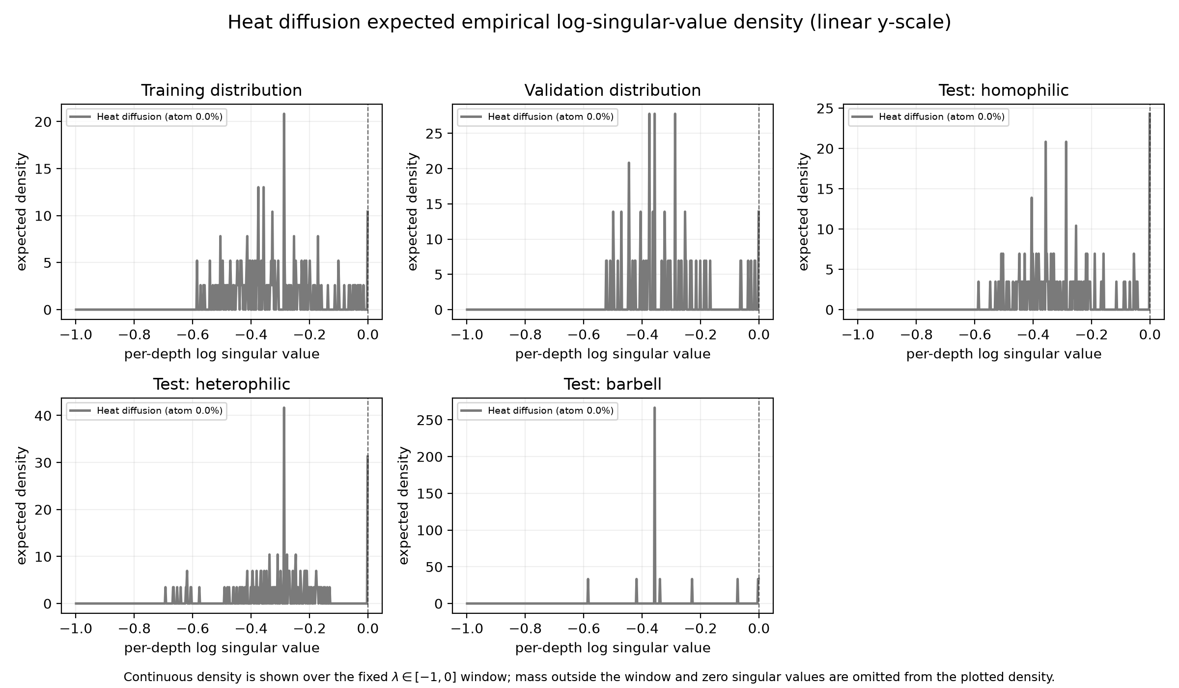
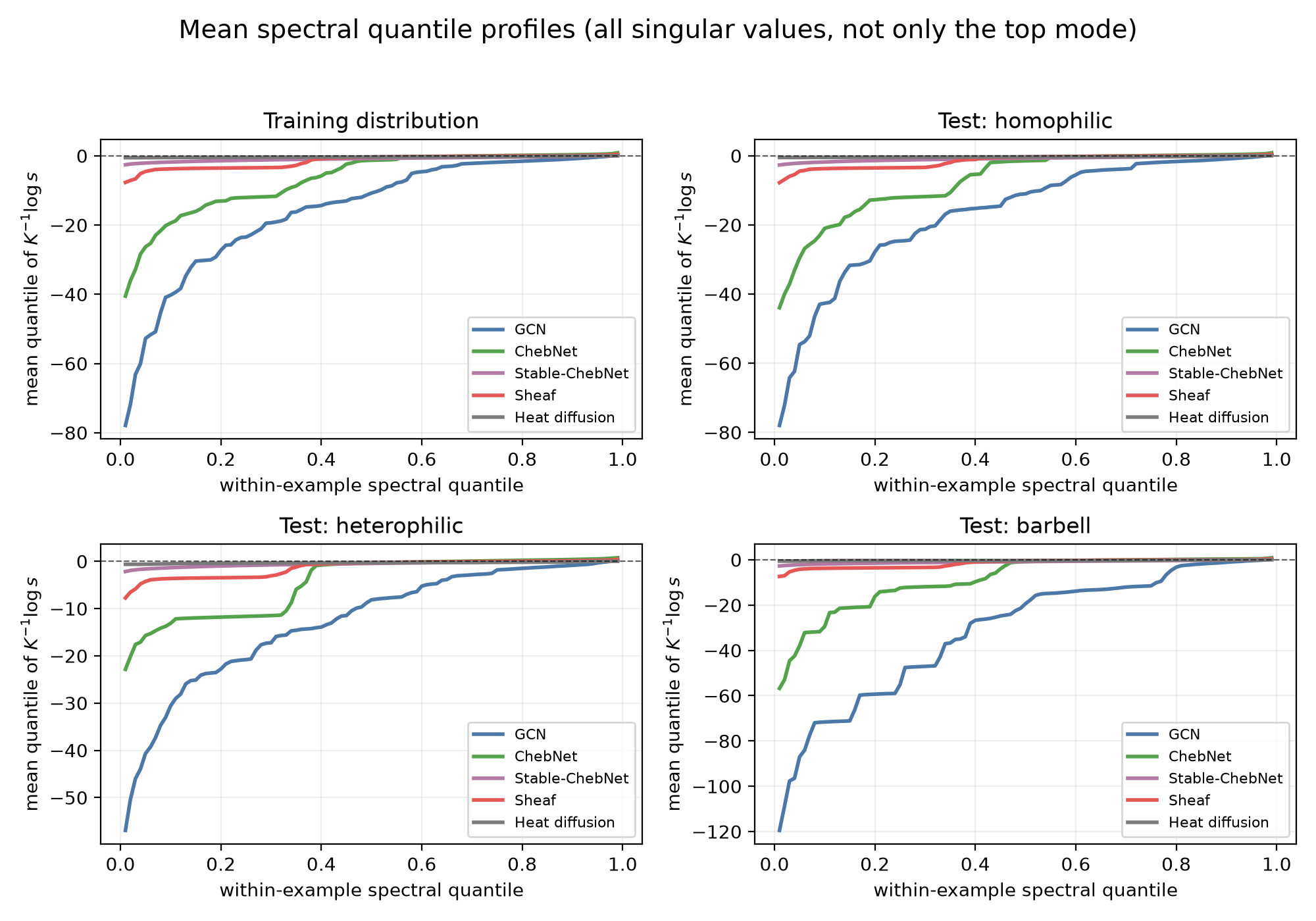
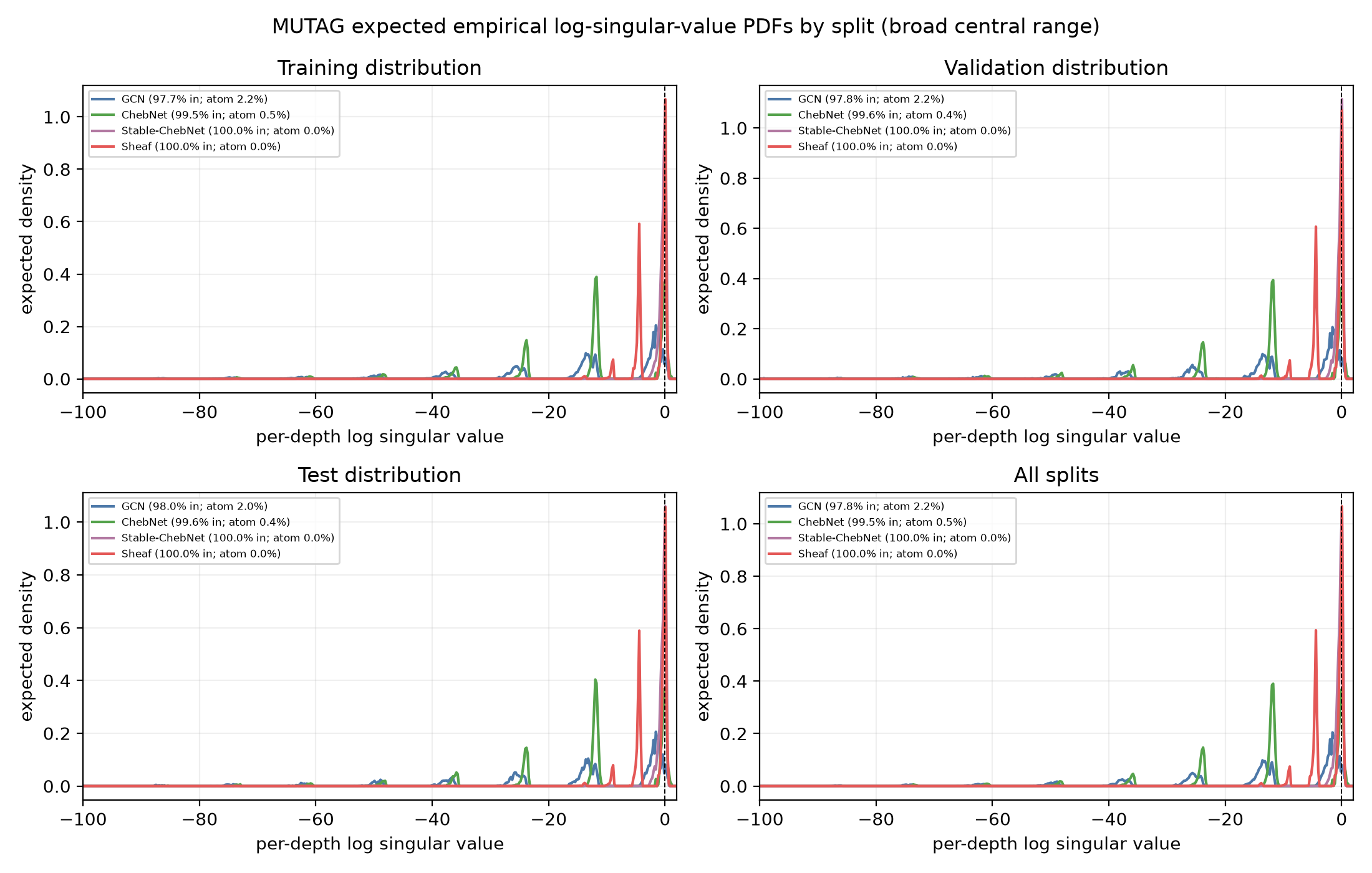
The expected measure is also split by the sign of its finite log-rates: positive mass corresponds to expanding singular directions and negative mass to contracting directions. Exact zero-rate mass and the separate zero-singular-value atom at −∞ are shown separately.

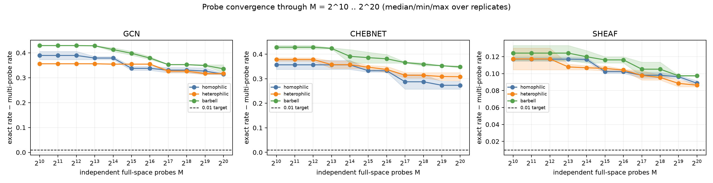
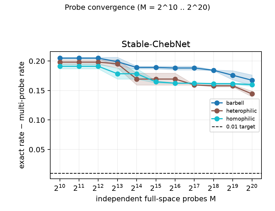
Expected empirical log-singular-value mass by sign for all systems and distributions — Expected mass in expanding, contracting, preserved, and zero-singular-value directions.

Probe convergence through 2^20 probes — Random-probe gap to the exact rate through M = 2^20 (1,048,576 probes): convergence is quasi-logarithmic and never reaches the 0.01 target.

Pushing probes from 2^10 to 2^20 closes only ~20% of the gap per 1024\times more probes (GCN 0.390→0.318, ChebNet 0.380→0.308, Stable-ChebNet 0.198→0.160, sheaf 0.117→0.090).

Stable-ChebNet probe convergence through 2^20 probes — Stable-ChebNet iid-probe convergence: the gap is smaller than for GCN/ChebNet here, but remains about 0.16 at one million probes.

Stable-ChebNet power and Lanczos speedup — Stable-ChebNet matrix-free speedups: early stopping is about 15× faster than fixed power and matches the exact reference.

Power-iteration speedup

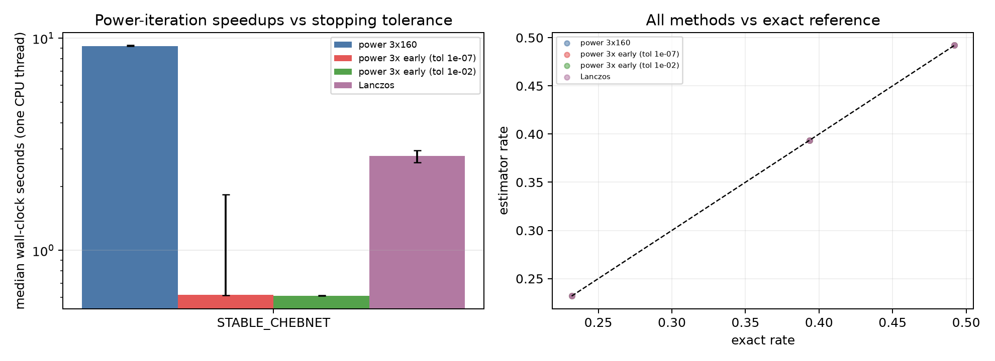
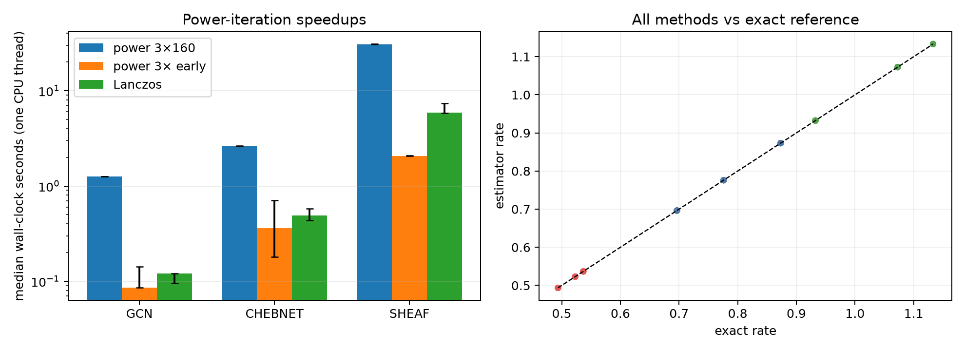
Two matrix-free upgrades are 5–15\times faster than the original fixed 3×160 protocol while matching the exact rate: early-stopping power (per-start stop at residual ≤10⁻⁷) and matrix-free Lanczos. Median per-cell wall-clock: sheaf 30.7 s → 2.06 s (early) and 5.9 s (Lanczos). Relaxing the stop threshold to residual ≤10⁻² buys additional speed only with fine-grained checks: at check_every=1 the residual hits 10⁻² by sweep 3, so per-cell times drop further to GCN 0.045 s, ChebNet 0.136 s, sheaf 1.09 s (~19–27× total, vs ~15× at 10⁻⁷), at a worst-case rate error ~10⁻⁴.

Power-speedup benchmark comparing 3x160, early-stopping power, and Lanczos — Median wall-clock and exact-rate agreement for 3×160, early-stopping power, and Lanczos.

Stable-ChebNet forward-only and adaptive follow-ups

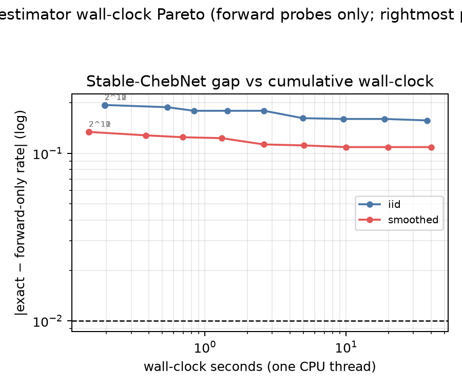
On the same three seed-90000 operators, Stable-ChebNet's graph-smoothed forward-only probes reduced the 2²⁰ gap from 0.157 (iid) to 0.109, at about 37.5–40.0 seconds. Adjoint-enabled refinement reduced the gap to 0.0021–0.0048 in two steps and below 10⁻⁴ in three to five steps. The frequency-adaptive forward-only tilt was worse than fixed smoothing at small budgets, with pooled gaps 0.20 versus 0.14 at M=10.

Stable-ChebNet forward-only wall-clock Pareto — Stable-ChebNet forward-only iid versus graph-smoothed probe wall-clock Pareto.

Stable-ChebNet random probes versus adjoint-adaptive refinement — Stable-ChebNet adjoint refinement converges in a few operator products where random probes remain far below the top singular rate.

Pierre's projected estimator

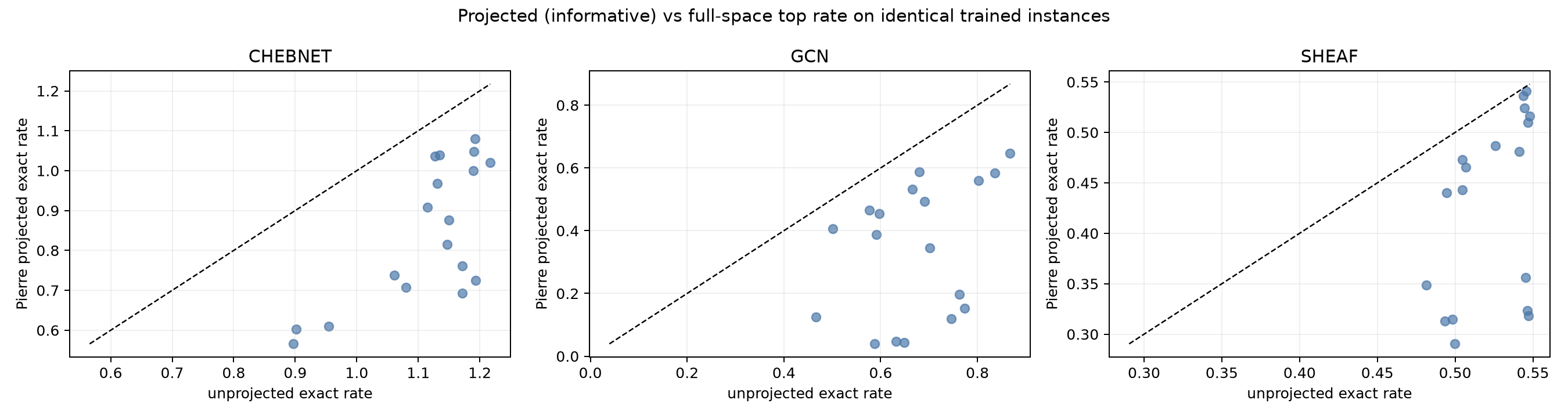
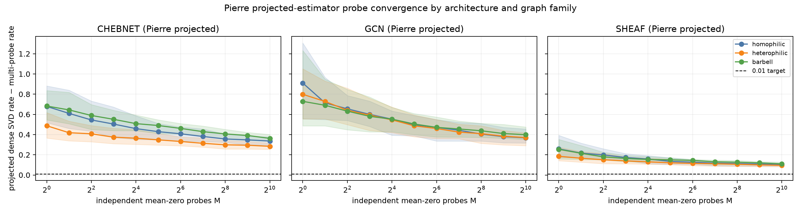
A separate experiment evaluates Pierre's deliberately different observable, which subtracts the node mean after every layer Jacobian action. Exact projected rates were lower than full-Jacobian rates on matched instances: mean GCN 0.344 versus 0.674, sheaf 0.427 versus 0.523, and ChebNet 0.844 versus 1.112. All 54 projected power-iteration cells passed the residual check and matched their projected dense-SVD references. Random projected probes still converged slowly and none reached the 0.01-per-layer target at 1,024 probes.

Pierre projected exact rates versus unprojected exact rates — Pierre's mean-zero projected observable is lower than the full-Jacobian rate, but remains positive on average.

Probe convergence for Pierre's projected estimator — Mean-zero projection does not resolve the slow convergence of independent random probes.

Recent spectral extensions

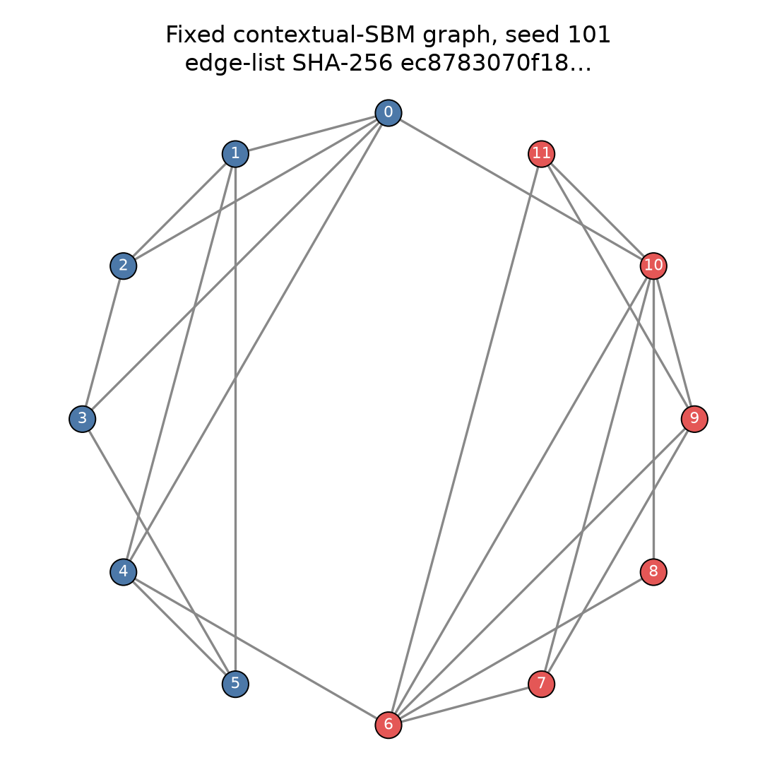
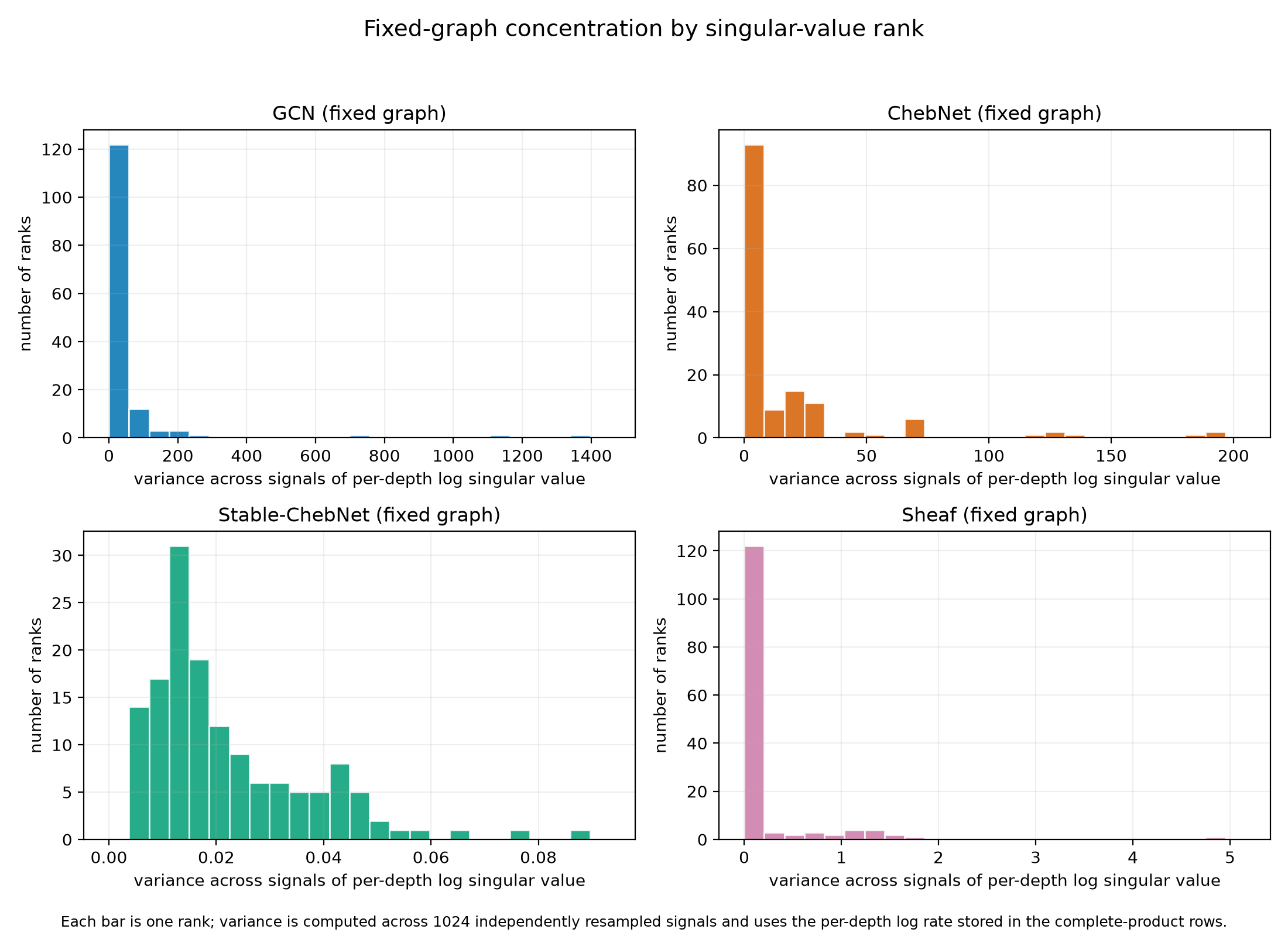
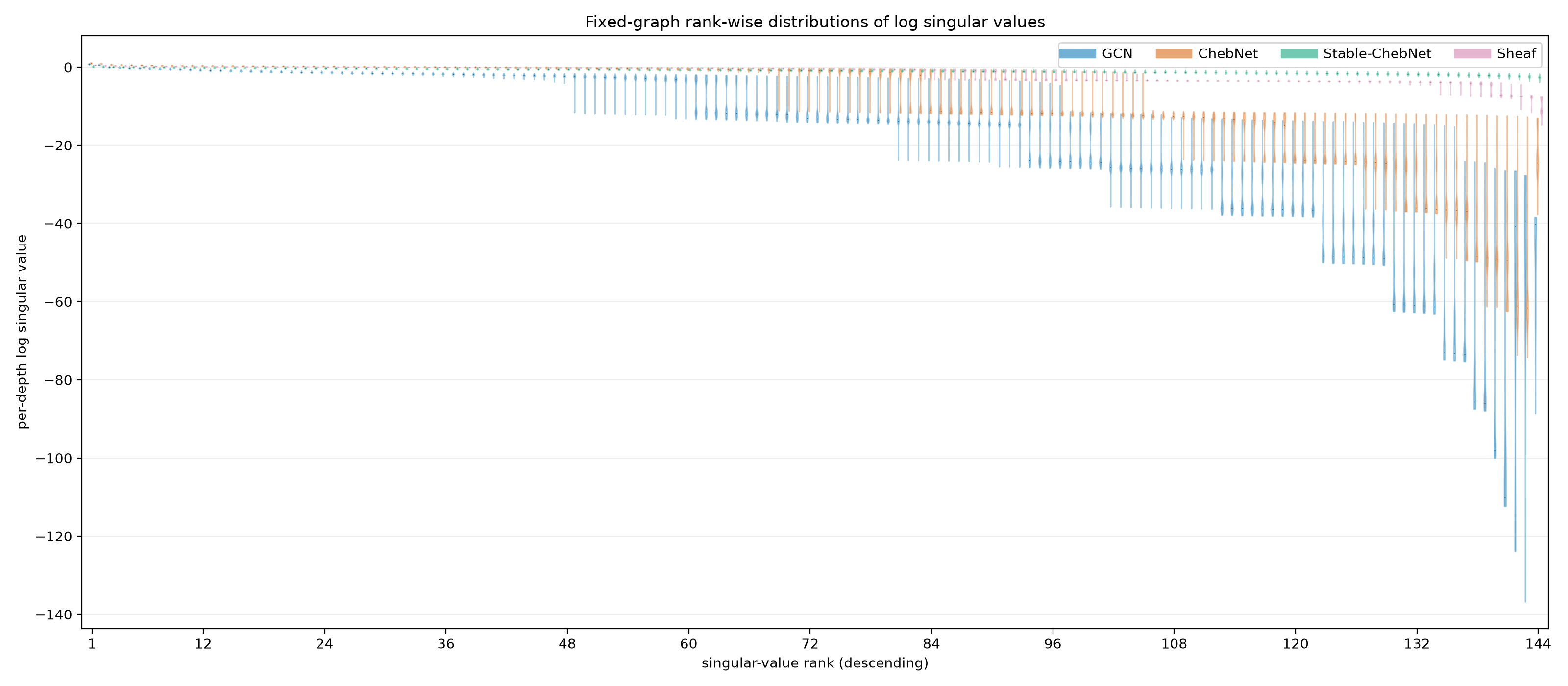
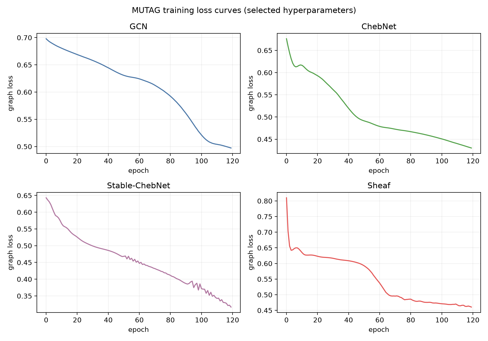
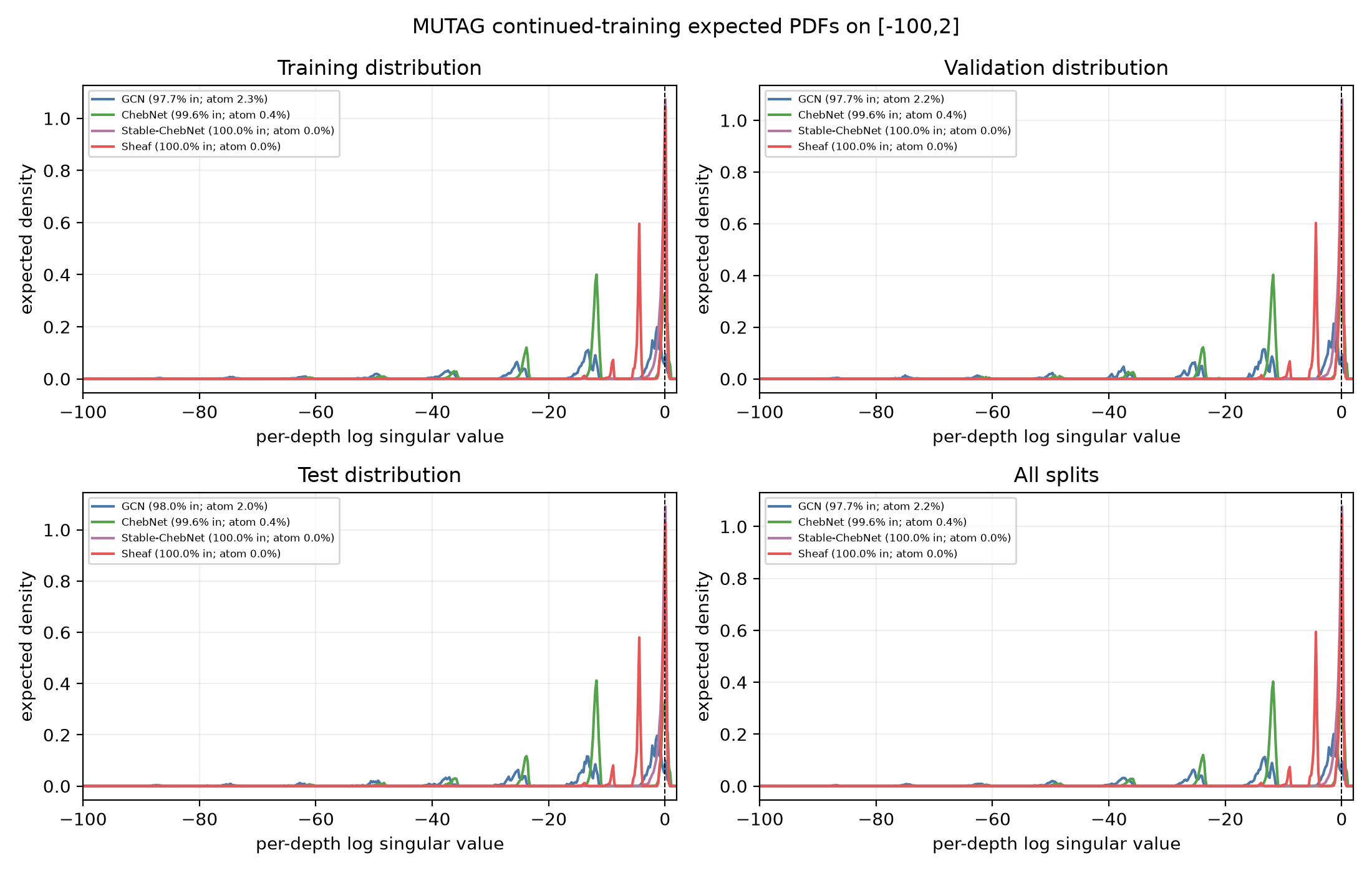
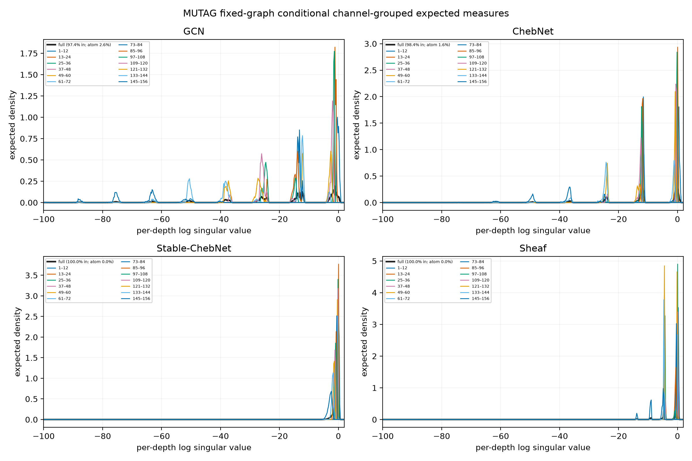
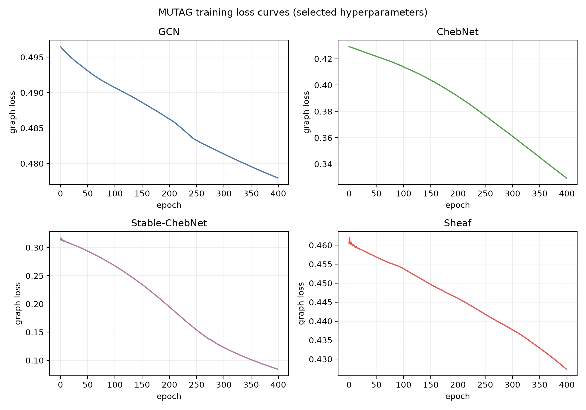
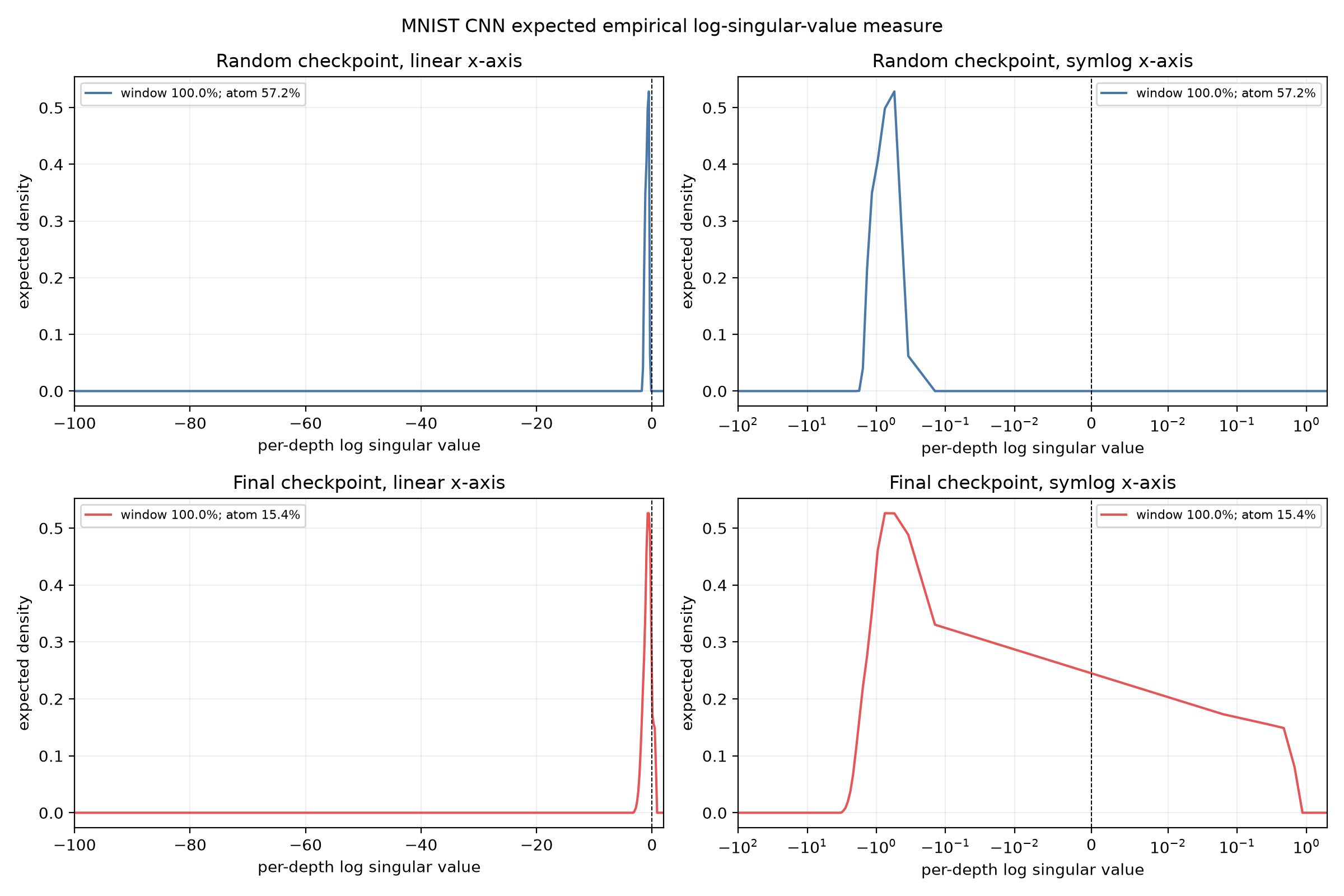
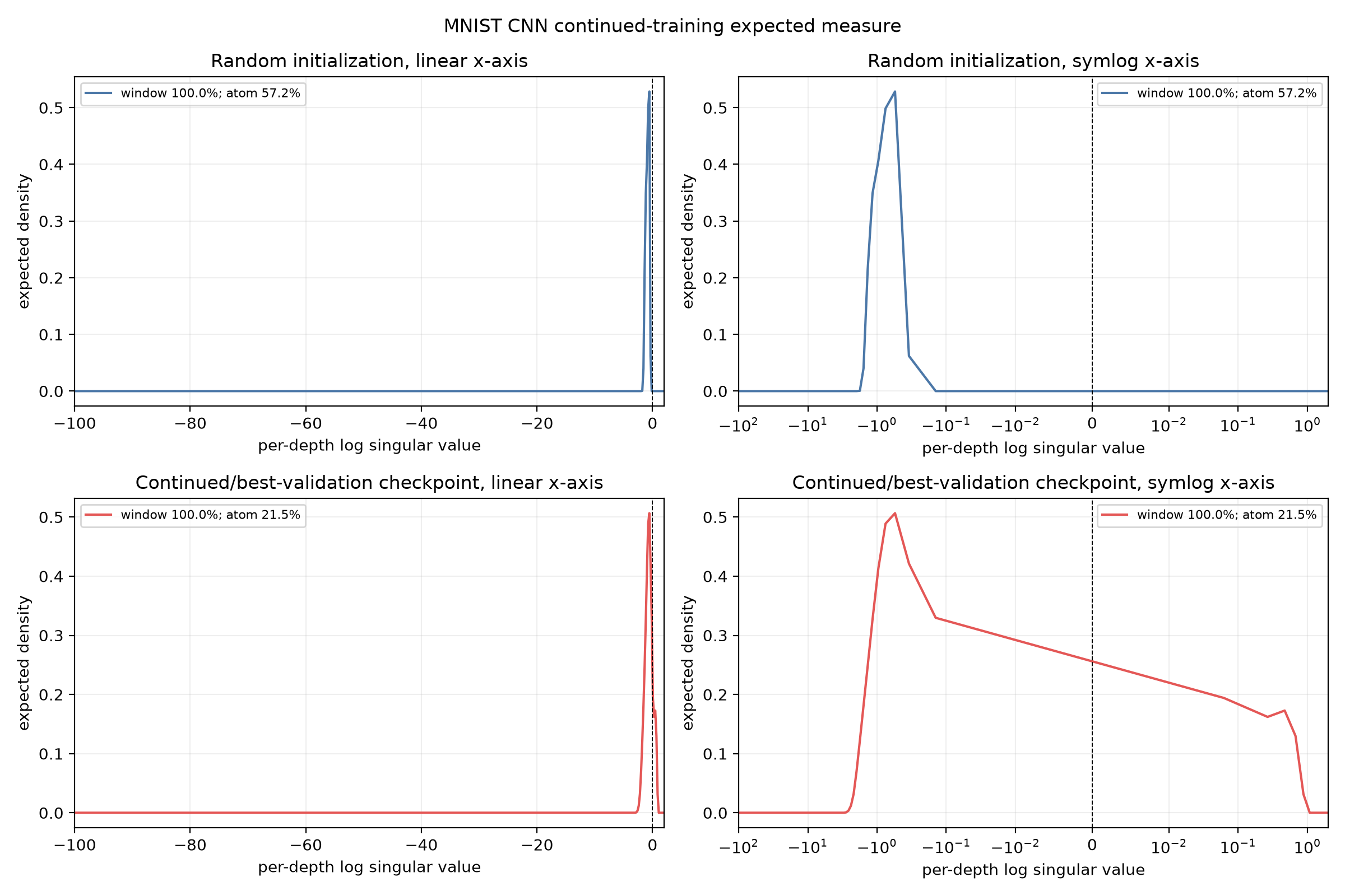
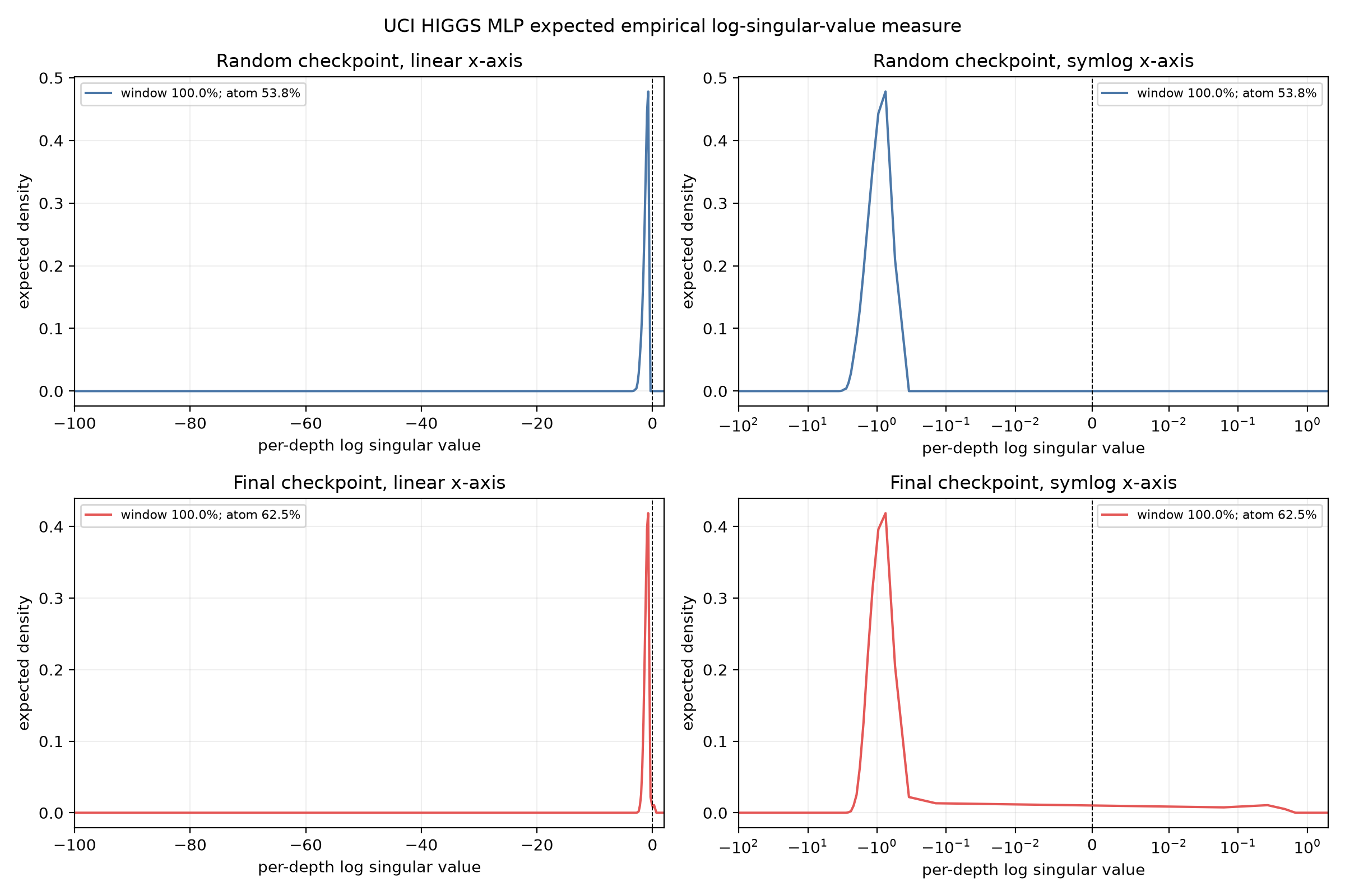
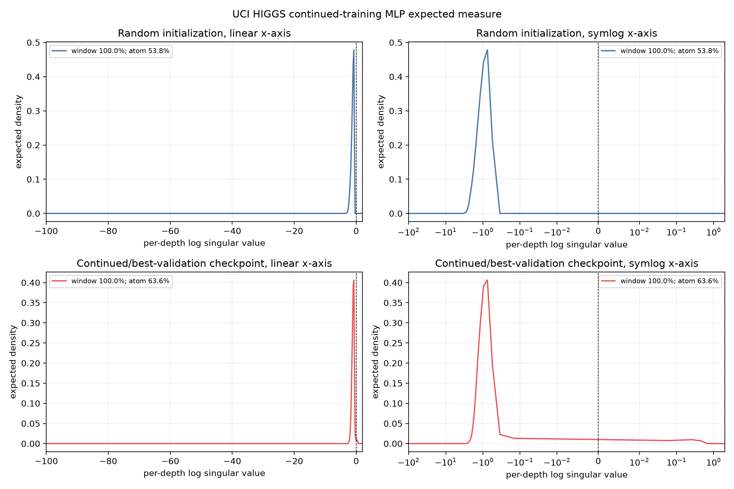
We now also condition the grouped spectral measure on one fixed graph while resampling signals, repeat the complete-product analysis on the MUTAG real-world molecular graph benchmark, and extend the expected-measure diagnostic to a no-pooling MNIST CNN and a four-hidden-layer 300-unit UCI HIGGS MLP. The complete 42-page report contains the full figure set, rank-concentration diagnostics, raw-singular-value checks, a 100-digit SVD precision control, continuation results, classification accuracies, loss curves, coverage/atom annotations, split details, and reproducibility manifests.

Fixed graph conditional grouped expected spectral densities — Fixed-graph conditional grouped expected measures with 1/(N C) normalization.

Fixed contextual SBM graph used for the conditional spectral experiment — Topology and class assignment of the fixed graph used for the conditional experiment.

Fixed-graph rank-wise variance histograms for log singular values — Rank-wise variance histograms across 1,024 fixed-graph signal resamples.

Fixed-graph rank-indexed violin distributions — Single violin plot showing all 144 singular-value ranks for all four GNN architectures.

MUTAG split-wise expected spectral PDFs for four trained GNNs — Split-wise expected empirical spectra on the MUTAG real-world graph distribution.

MUTAG GNN training loss curves — MUTAG graph-classification loss curves for the four selected models.

MUTAG continued-checkpoint expected spectral PDFs — Expected MUTAG spectra after 400-epoch continuation and best-validation checkpoint selection.

MUTAG continued fixed-graph grouped spectral densities — Continued MUTAG fixed-graph grouped spectra with six high-contrast cycling colors.

MUTAG continuation loss curves — Continuation loss curves; the reported checkpoint is selected by validation accuracy.

MNIST CNN random and final expected spectra with linear and symmetric-log x axes — MNIST CNN expected spectra for random and final checkpoints on linear and symmetric-log x axes.

MNIST CNN continued expected spectra — MNIST spectra after 20-epoch continuation: validation accuracy improves from 0.9205 to 0.9410.

UCI HIGGS MLP random and final expected spectra with linear and symmetric-log x axes — UCI HIGGS MLP expected spectra for random and final checkpoints on linear and symmetric-log x axes.

UCI HIGGS MLP continued expected spectra — HIGGS spectra after 40-epoch continuation: validation accuracy improves from 0.7159 to 0.7185.

Recommended practice

For small calibration cases, validate JVP/VJP products against a dense reverse-mode Jacobian and SVD.
For the scalable finite-depth top rate, use multiple-start power iteration on the full unprojected Jacobian product; report residuals and do not accept nonconverged runs.
Use random probes as labeled lower bounds or spectral-shape diagnostics, after calibration; do not silently treat a fixed probe count as the exponent.
Do not insert a mean-zero projection when claiming to measure the full Jacobian: it changes the operator. If scientifically useful, report Pierre's projected cocycle as a separately named observable.